Data Visualization with ggplot
Data Visualization
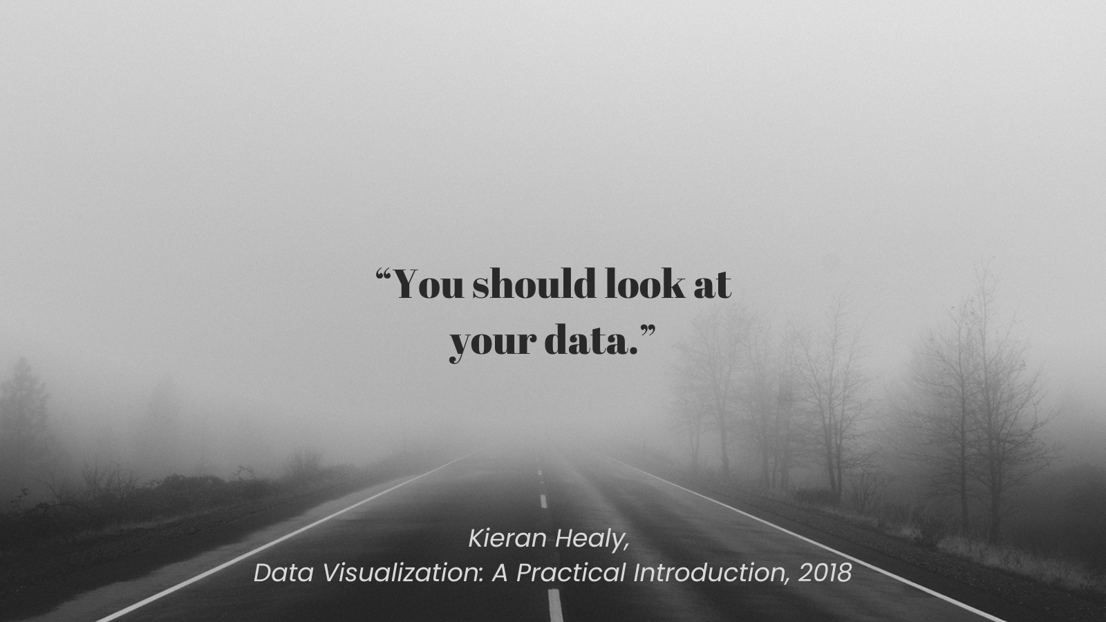
Exploration
Look at distributions
Examine relationship between variables
Communication
Illustrate your findings in ways that are digestible
Make or support an argument
The Grammar
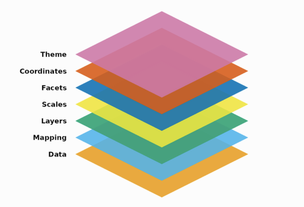
“In brief, the grammar tells us that a graphic maps the data to the aesthetic attributes (colour, shape, size) of geometric objects (points, lines, bars).”
Hadley Wickham
Data
- Data - information used to create the graphic

Aesthetic Mappings
- Aesthetic attributes - x, y, color, size
Layers
- Geoms- geometric representations of the data
Scales
Scales - translate what is in the graph to what is in the data using legends or axes
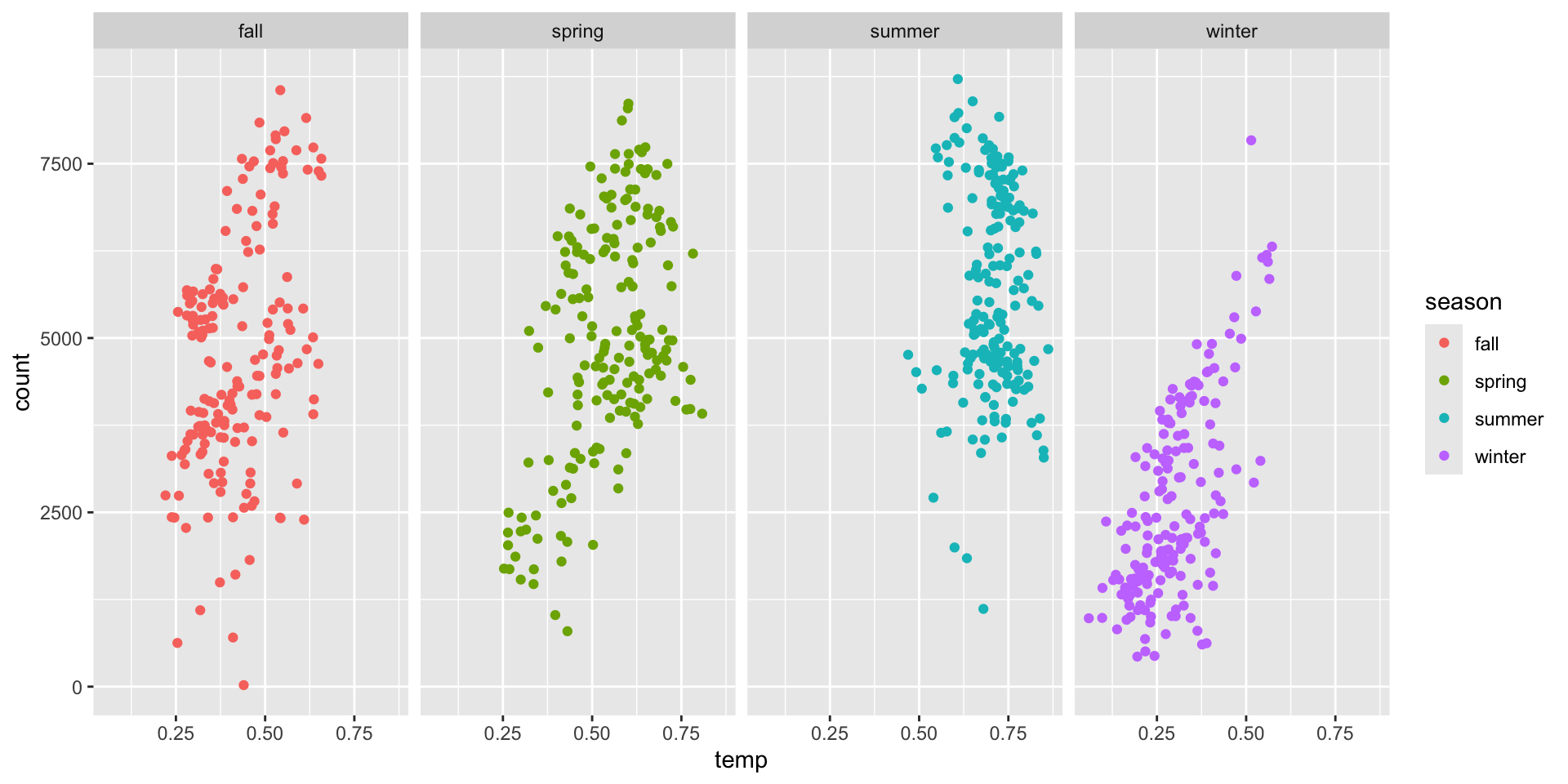
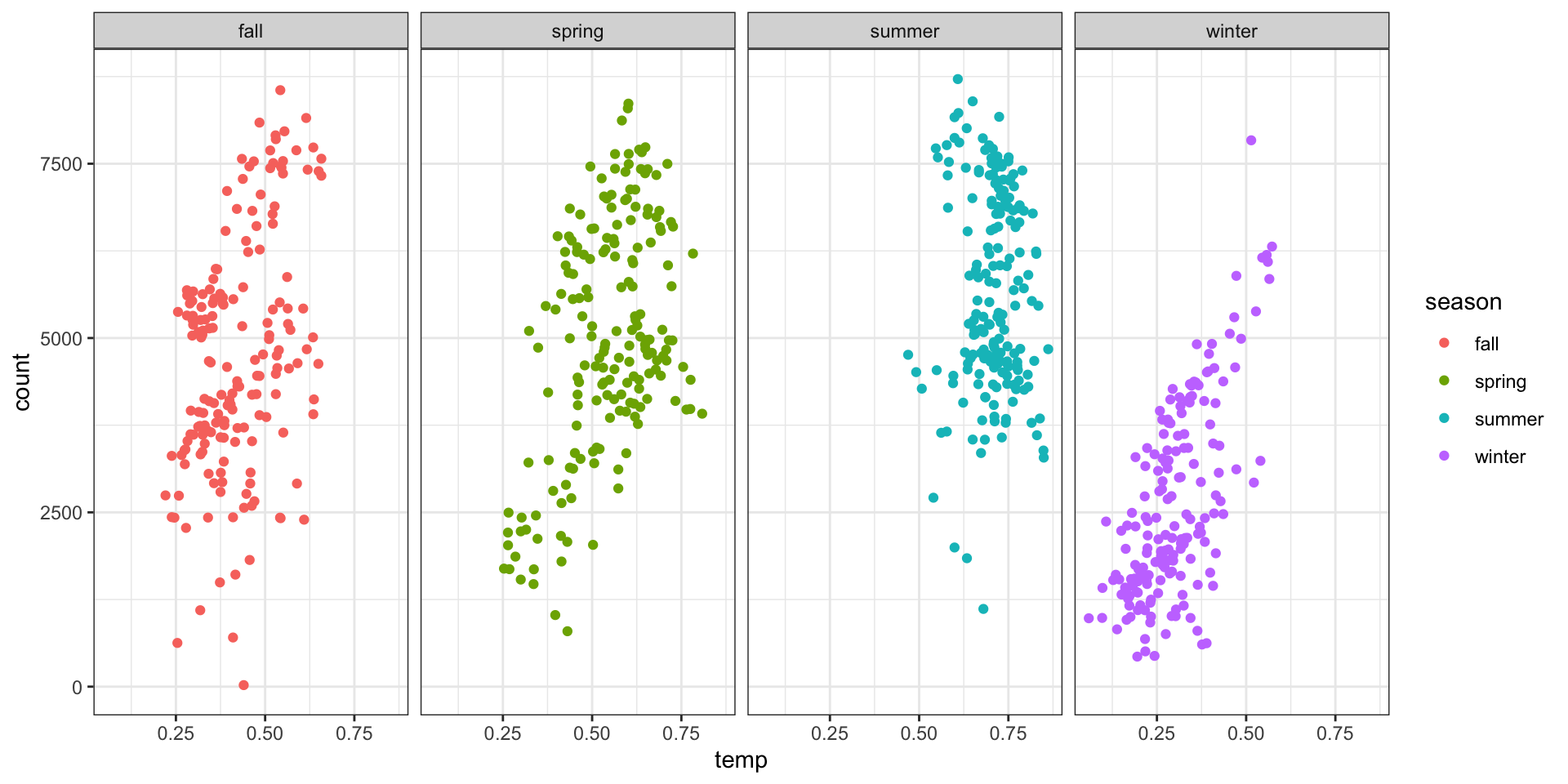
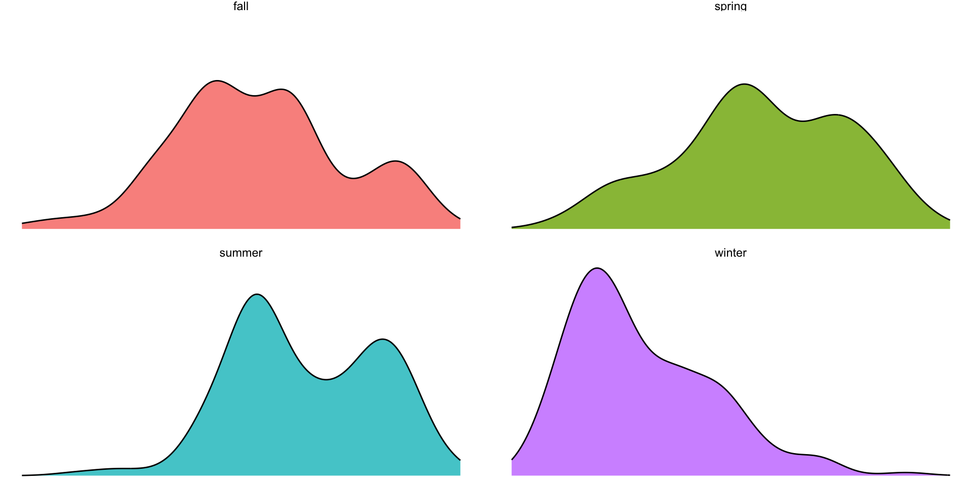
Facets
- Facets - small multiples
Theme
Theme - set overall how the graph looks
Cleaning Up
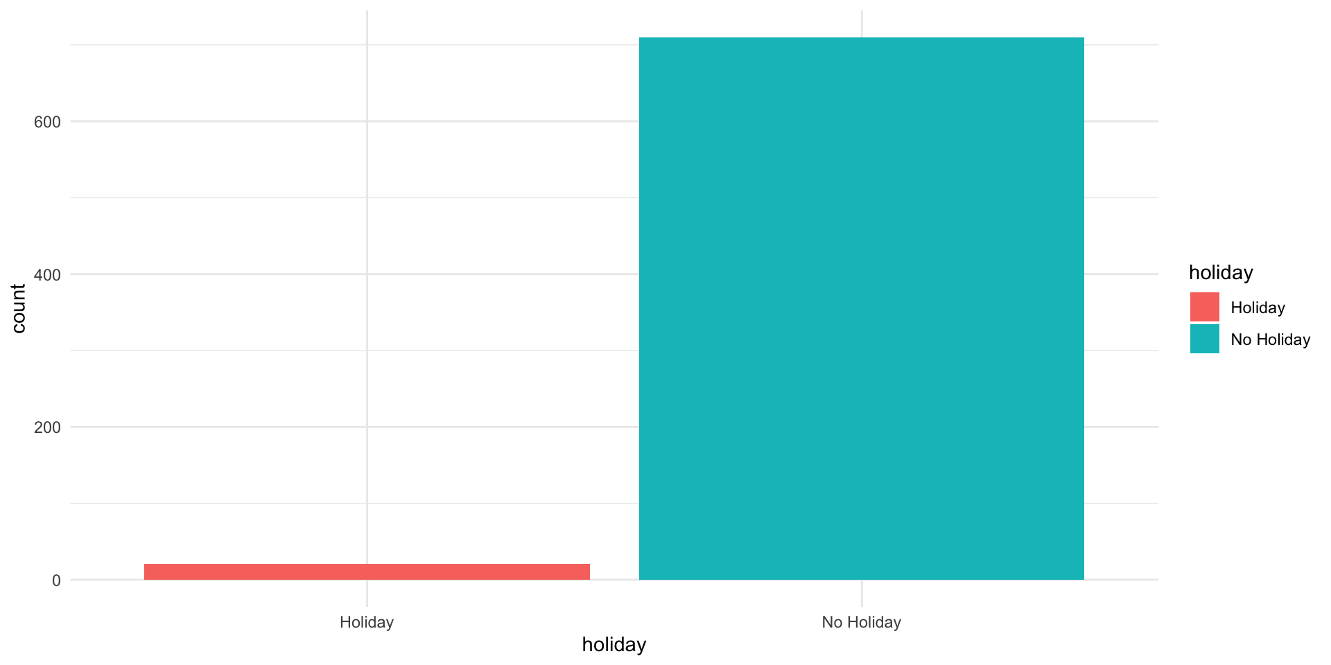
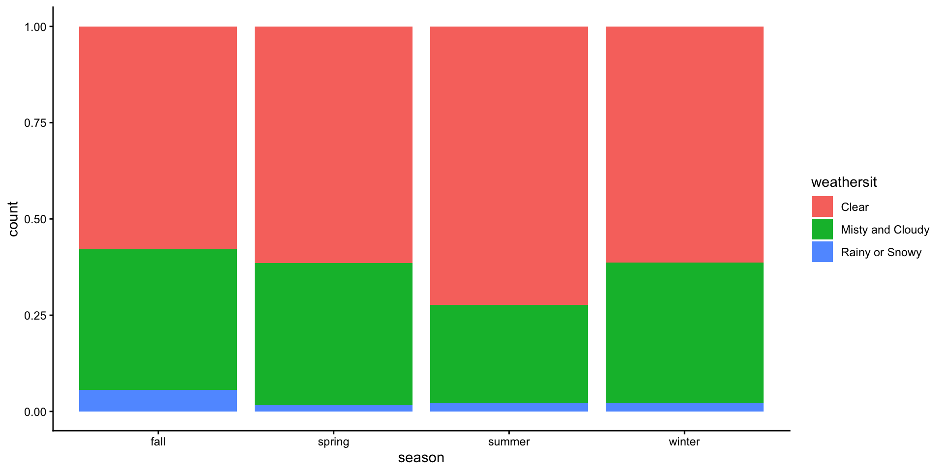
Bar Plot: Categorical Data
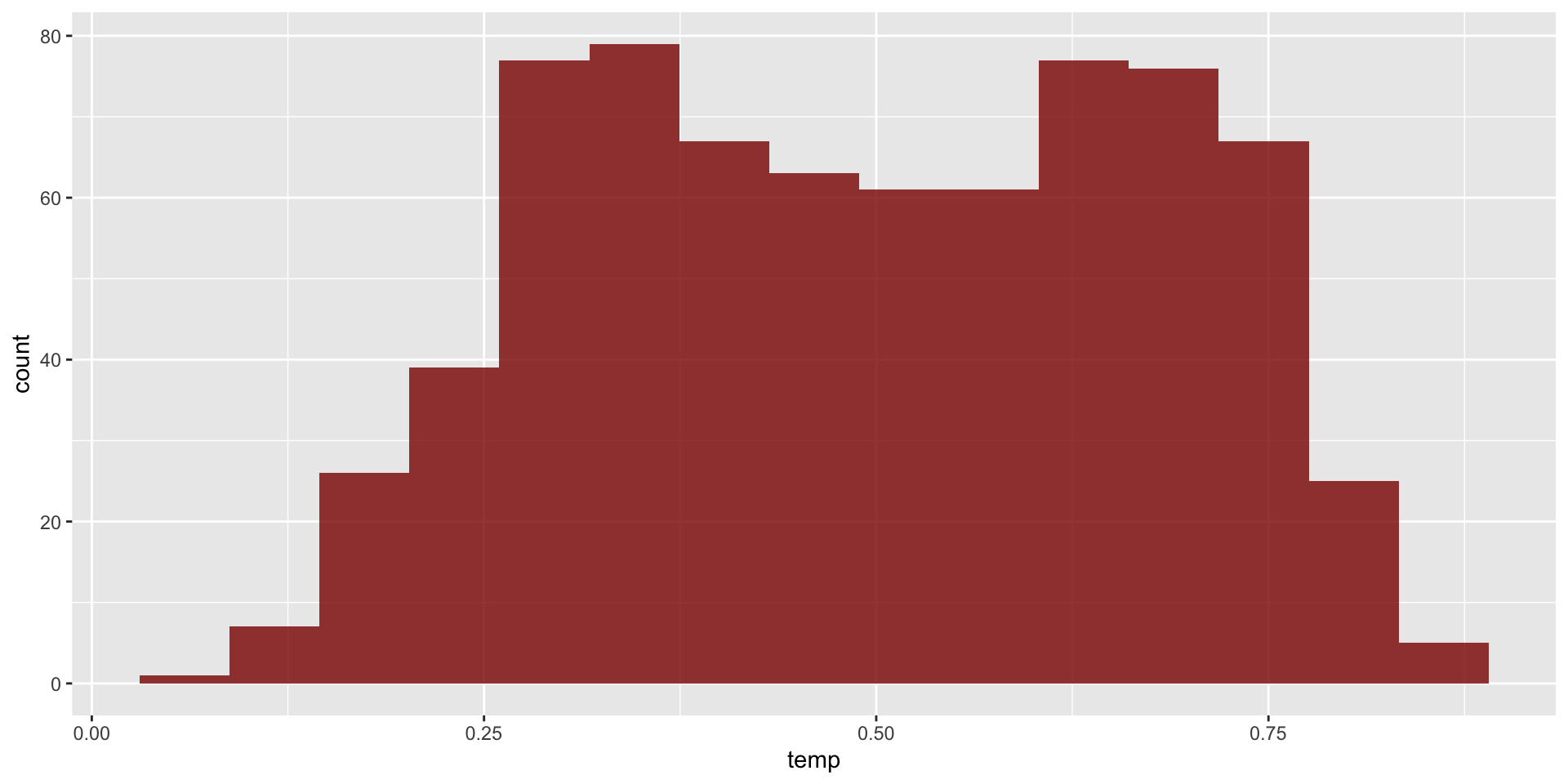
Histogram: Continuous Data
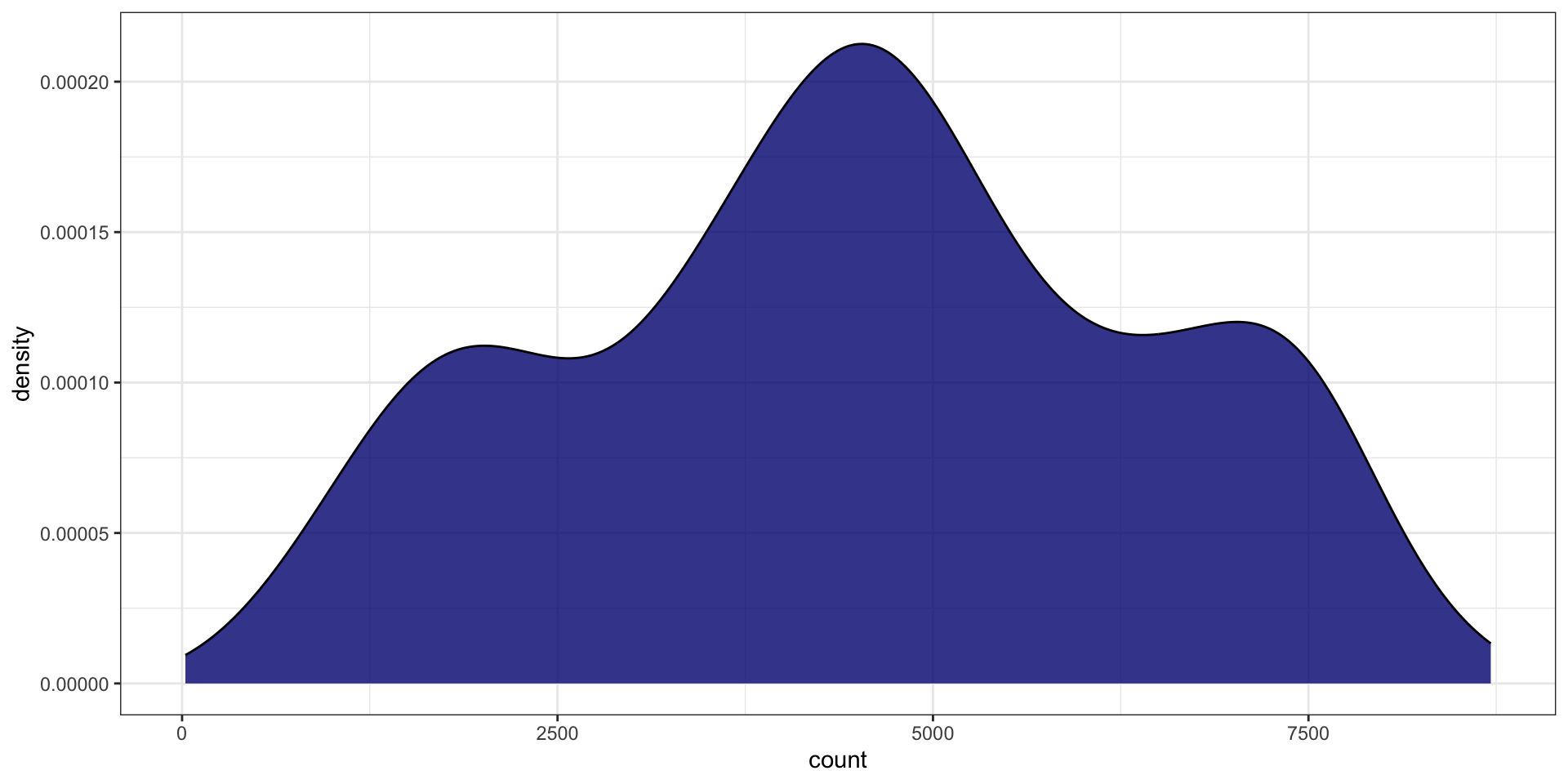
Density Plot: Continuous Data
Bar Plot: Categorical Data
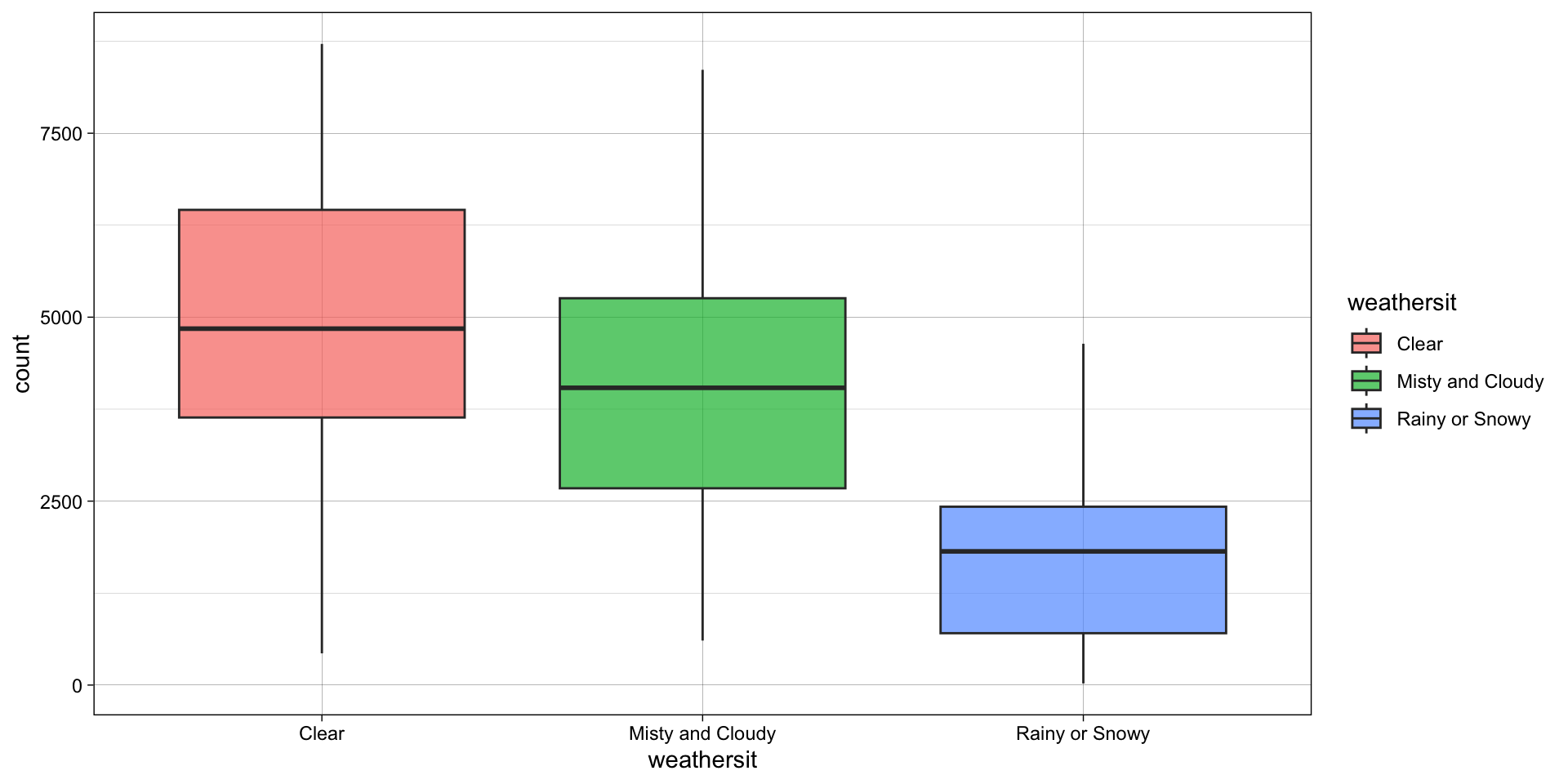
Box Plot
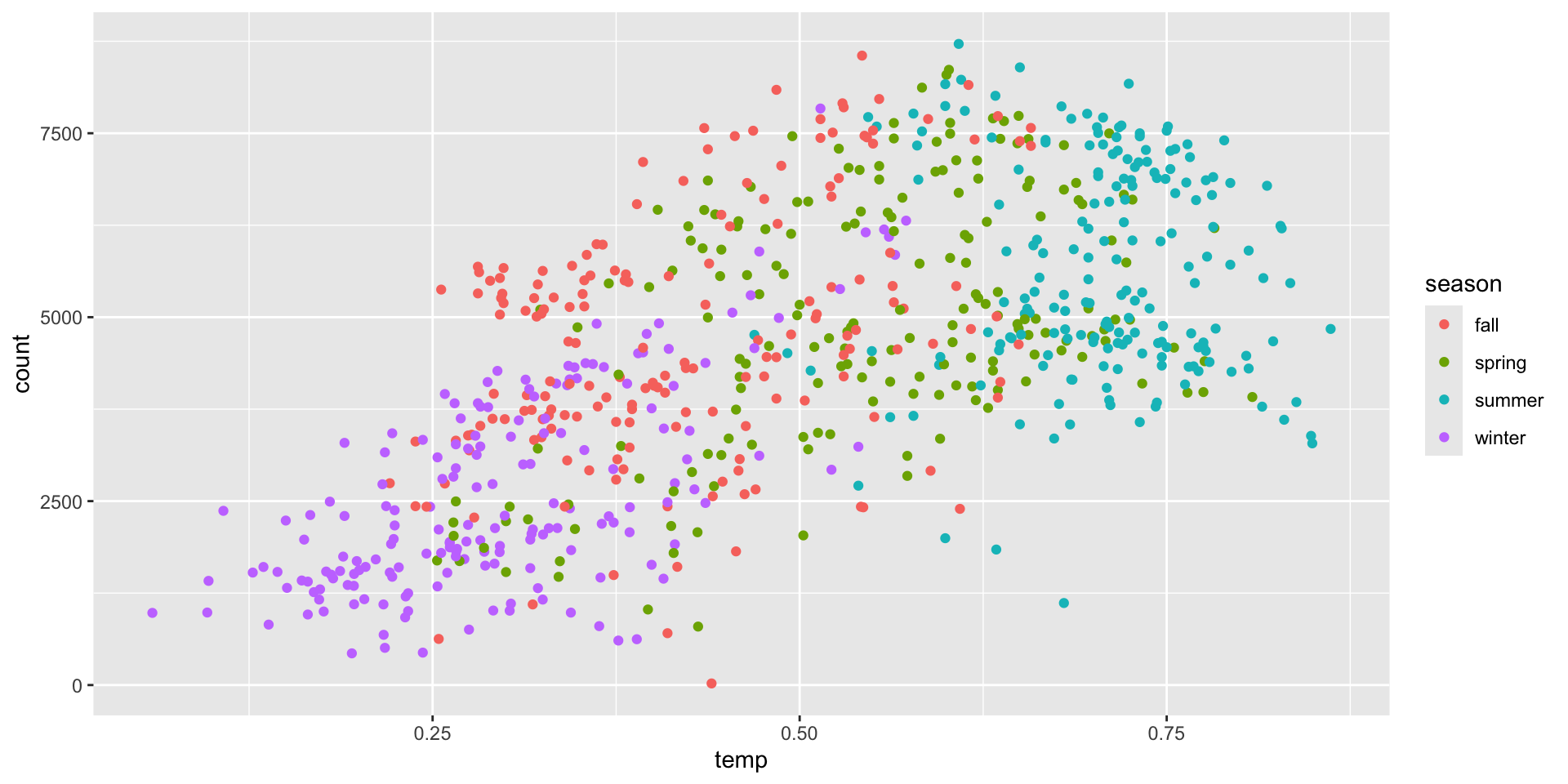
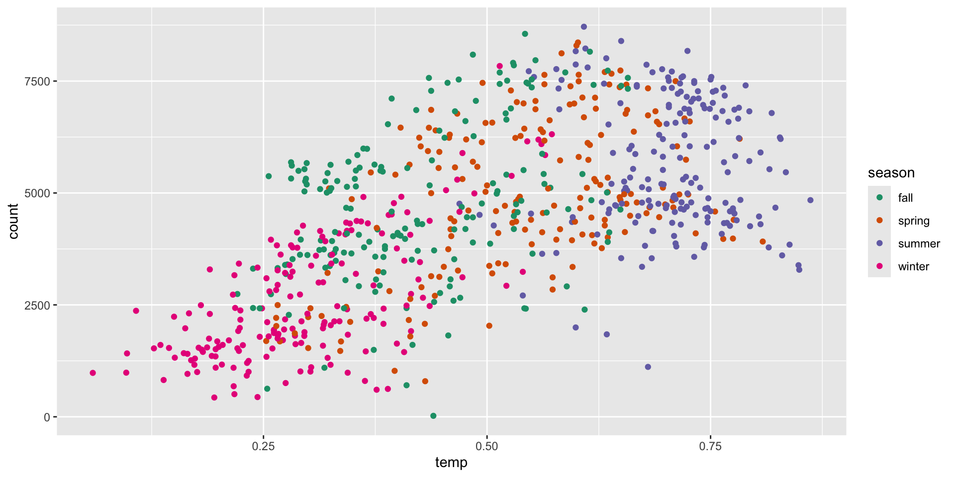
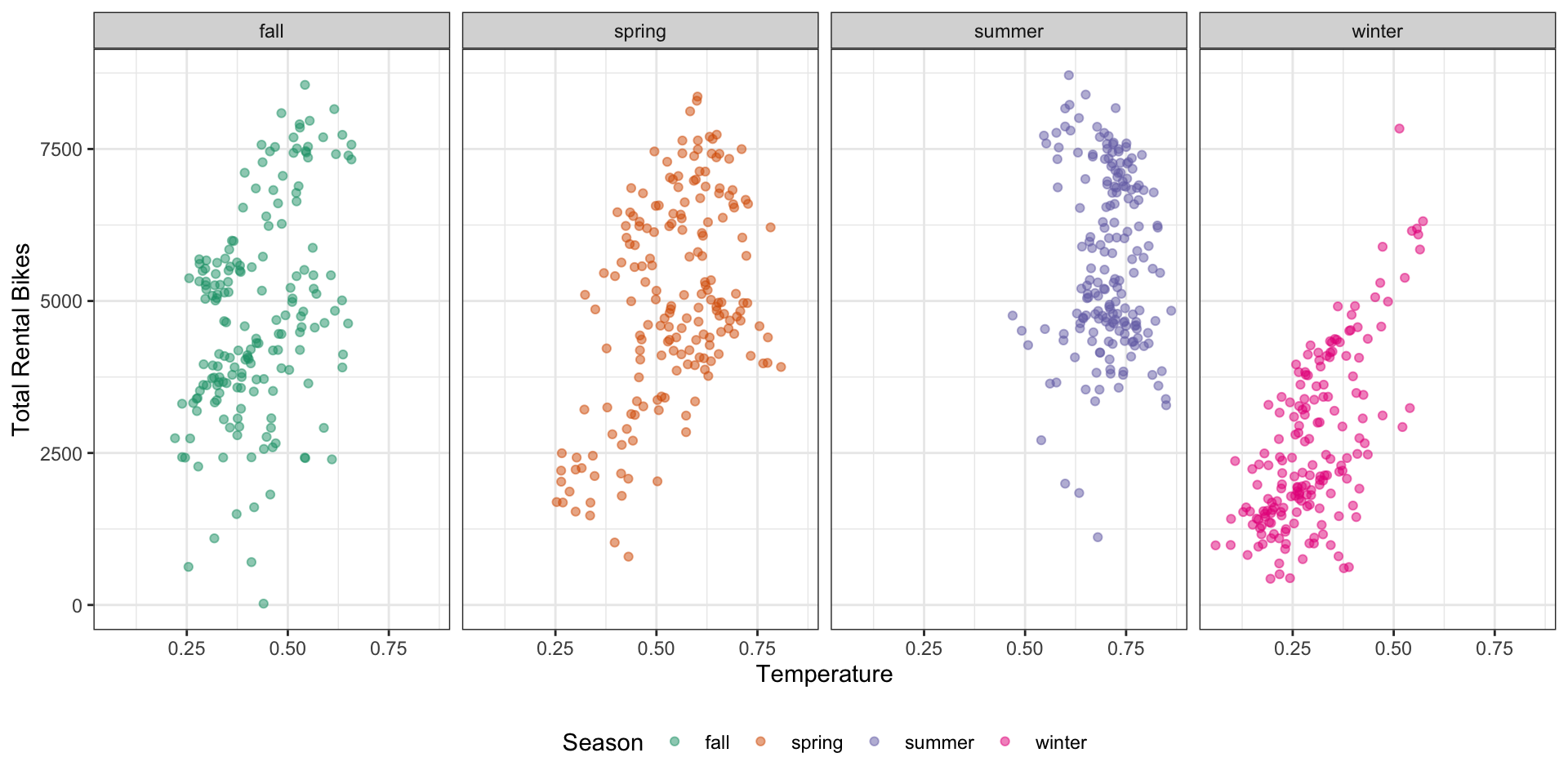
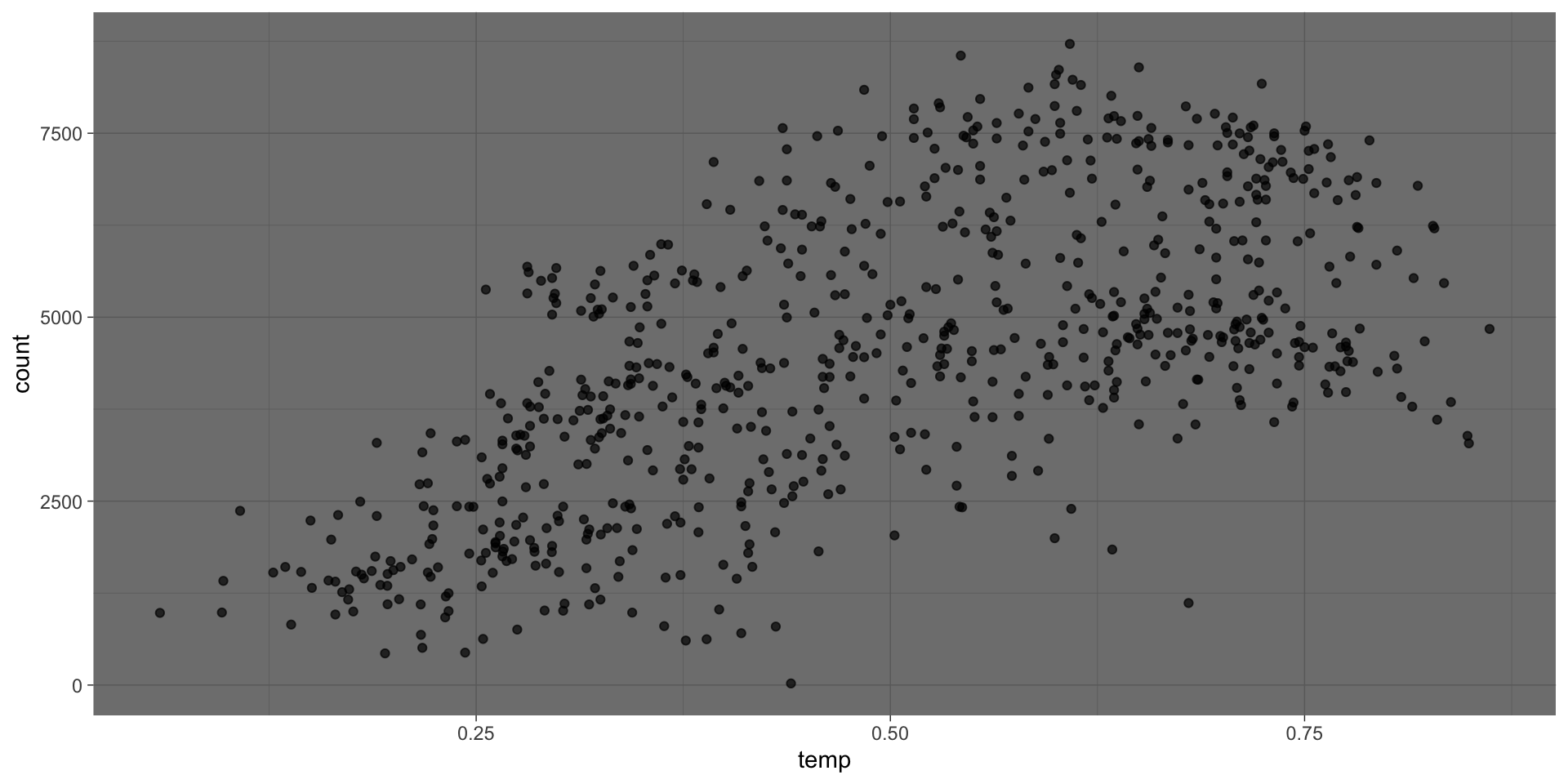
Scatter Plot: Continuous Data
Total Rentals by Season
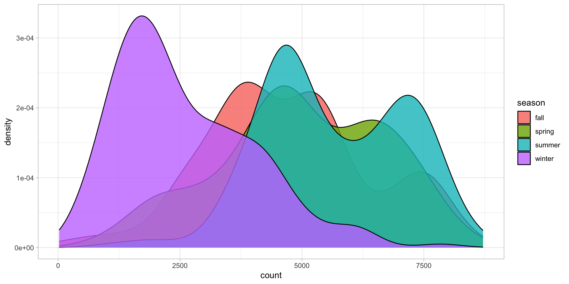
Total Rentals by Season
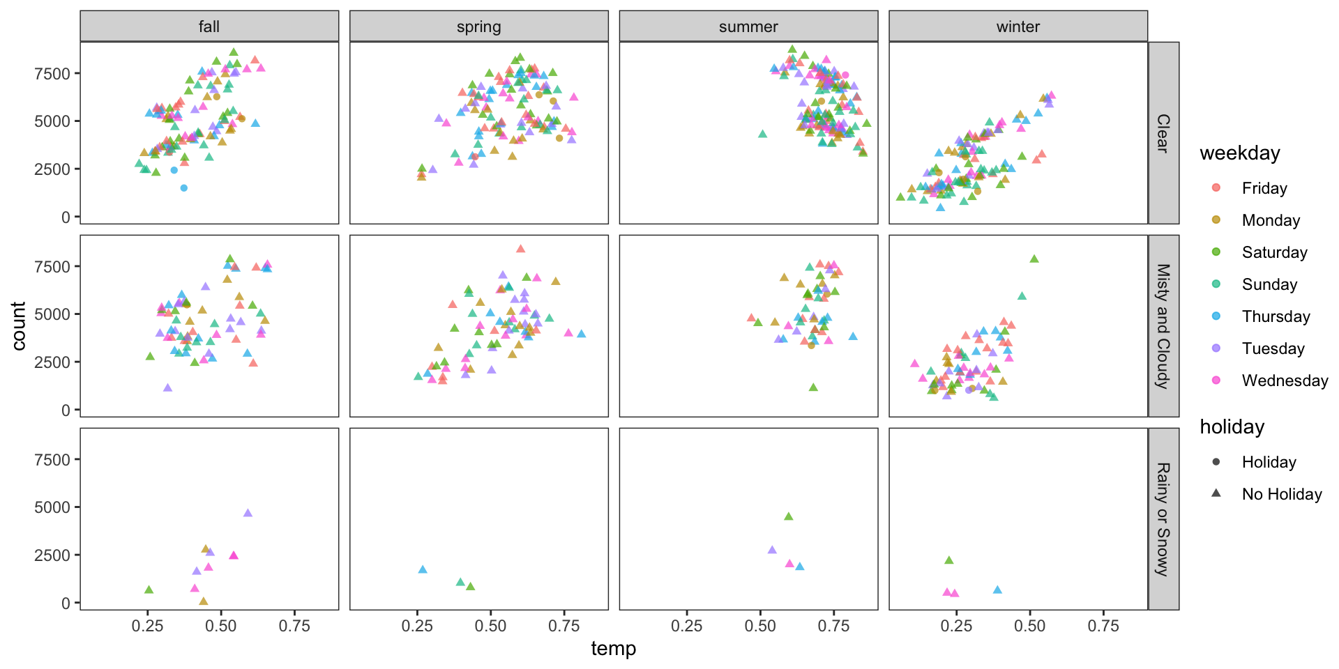
Relationship Between Temperature and Total Rentals by Season and Weather and by Weekday and Holiday